Traveling Salesman Problem

TSP Algorithms

The visualizations shown below grew out of the difficult personal experience of tightly budgeting a long backpacking trip through Europe. To save money, it seemed advantageous to travel in the manner of a greedy algorithm, optimizing for distance (i.e. going to the first closest destination, then all successively closest destinations). The logic assumes that to minimize the distance is also to minimize the overall travel cost. In reality, however, there are several factors which could confound this assumption: promotional travel deals, seasonal price variations, and unusual transportation routes, amongst others.

A brief look into the problem area showed me that I'd come across a variation of the Traveling Salesman Problem (TSP). The problem asks, "Given a list of cities and distances between them, what is the shortest way for a salesman to visit each city exactly once and return to the original city?" My version simply replaces "distance" by "cost to visit" and is a mathematically identical formulation. Therefore, I gathered travel cost data between the 21 cities I planned to visit, and began to solve the problem. I used two basic optimization approaches: a greedy algorithm and the 2-Opt algorithm.

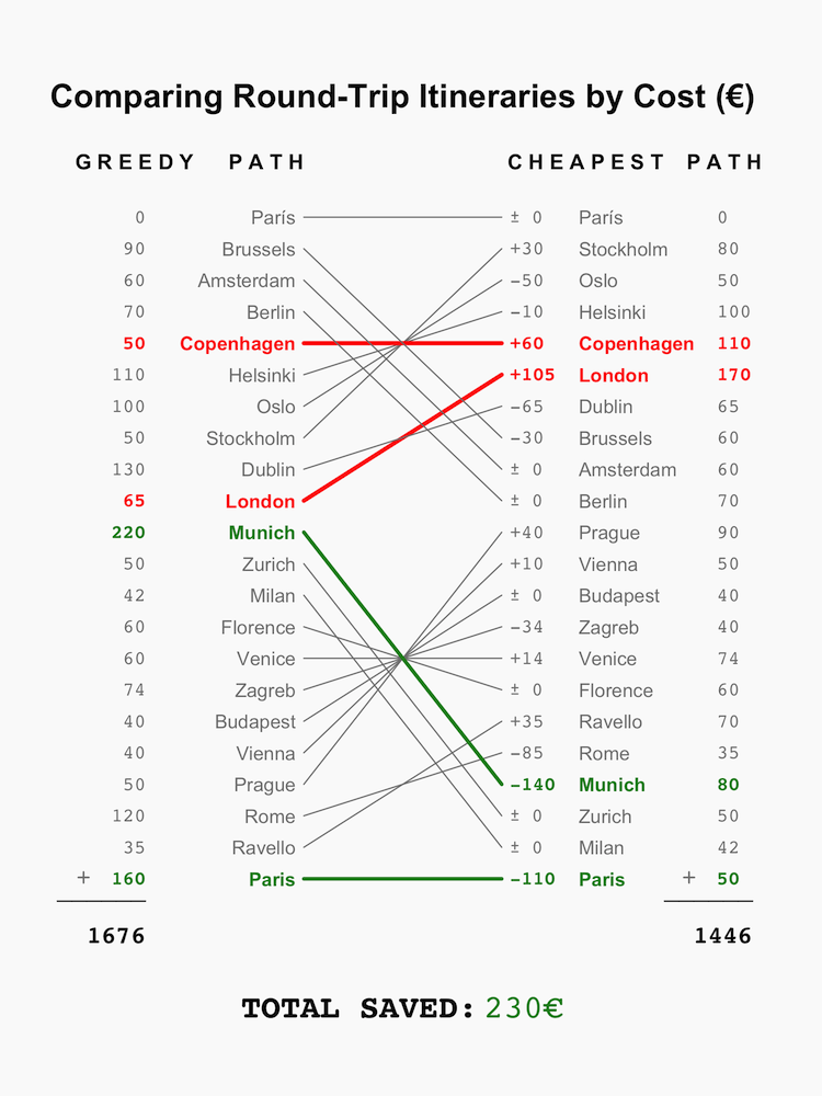
Greedy Algorithm: This optimization procedure simply took my city of origin, Paris, and initially went to the cheapest place, Brussels. Then, it successively went on the cheapest trip to the next city, ending with a trip that would cost 1676€. This was a decent start, but the nature of the greedy algorithm is myopic and ends at a local minimum with no guarantee of having found the optimal solution. This led me to 2-Opt.

2-Opt: The 2-Opt solution to the TSP aims to fix the narrow sight of the greedy algorithm by doing a corrective survey of the initial greedy groundwork. Visually, any two paths that would cross each other in the greedy solution get uncrossed, and if the change results in a cost improvement, the swap is kept. Therefore, a functional 2-Opt solution can at best improve upon the local minimum found by the greedy algorithm, and at worst, be the same.

TSP Slopegraphs

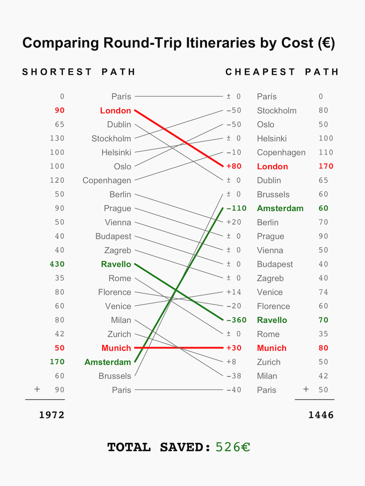
The slopegraphs found below show a bit of the work I put into creating a useful visualization of different possible paths through Europe. Visually, the highlighted paths in green represent the best cost saving swaps. On the left, for instance, we find that going to Ravello from Florence is 360€ cheaper than going from Zagreb. Vice versa, the higlighted red paths represent swaps that lose money - on the left, getting to London from Copenhagen instead of Paris is more expensive.

The visualization on the left aims to show that the shortest path through these 21 European cities, as found by the 2-Opt algorithm minimizing distance, is a much more expensive option than the cheapest path, as found by 2-Opt algorithm minimizing cost. On the right hand side, the visualization demonstrates that the greedy algorithm's path, while somewhat effective, also does not result in the cheapest path. Instead, it can and should be tweaked to save some money. For a traveler on a tight budget, finding even these small savings can make all the difference on a trip.

TSP Assumptions

In order to create the visualizations, I made a few assumptions about the data that simplified the problem, making it more of a theoretical and visual exercise than a practical solution to the travel planning issue. Here are a few of the more pressing limitations.

Monthly Averages: I chose to collect travel cost data between these cities only for the month of September in 2015 because it was most readily available. I used Google Flights, Rome2Rio, RailEurope and Eurolines as my sources and simply took monthly averages of the cheapest transport option on each day. This gives a poor picture of true cost since costs fluctuate by days, weeks, months, seasons and are subject to special offers.

Scheduling: In a similar vein, the use of monthly averages does not incorporate the issue of planning in almost any way. I did not try to account for the number of days that might be spent in any location, so the travel costs do not reflect a true schedule.

Symmetry: Lastly, I assumed that traveling from A → B costs the same as B → A, a symmetry that does not always exist in the real world. While this made the data collection and mathematics simpler, it is not a true reflection of travel costs.